By using a columnar layout for vectors, you can speed up vector similarity search thanks to the more efficient distance kernels and efficient pruning of dimensions.
This entry is a summary of our work, PDX: A Data Layout for Vector Similarity Search.
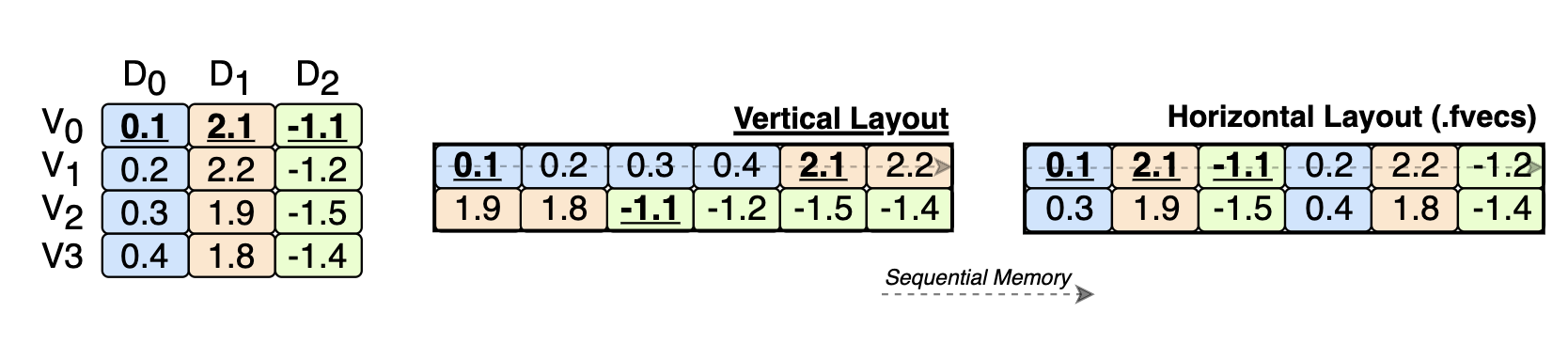
A few months ago, we came across this 20-year-old paper proposing a vertical layout for vectors. That means not storing vectors one after the other but storing the same dimension of different vectors together (see image above). In databases, this is referred to as “columnar storage.”
Fast-forward 20 years, this idea has been used (up to some extent) to speed up lookups on product quantized (PQ) vectors. However, we saw a broader potential in this idea. Would it be useful in other modern vector similarity search algorithms? From there, we started working on PDX (Partition Dimension Across), a vertical layout for vector similarity search.
In principle, it seems like a meaningless change. How can transposing the vectors help vector similarity search? The key observation is that in the vertical layout, a search happens dimension-by-dimension instead of vector-by-vector. With this in mind, distance kernels used in vector similarity search (Inner Product in the following example) now look like this:
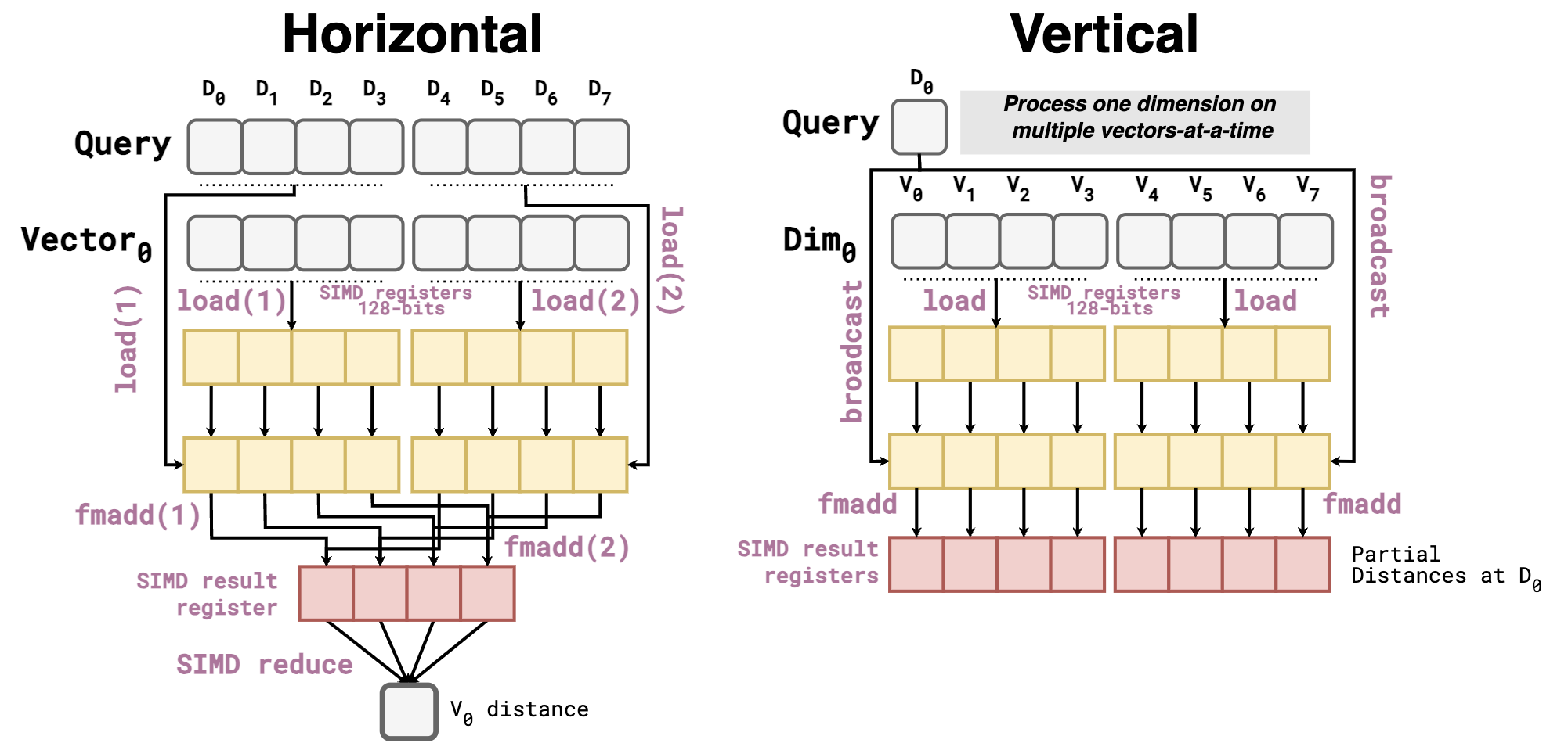
The vertical kernel has a lot of advantages over the horizontal one:
- Zero dependencies, as the distances of different vectors (
redboxes) are aggregated in different SIMD lanes. Thus, allowing the work to be fully pipelined. Contrary to the horizontal kernel, in which the result of the secondFMADDdepends on the previous one. - No reduction step of the SIMD register, as the distance of each vector is already aggregated in different SIMD lanes.
- Efficient even at low dimensionalities. If I use a CPU with AVX512 (512-bit registers that fit 16
float32), and my vectors have a dimensionality of 12, every call toFMADDwould waste 4 SIMD lanes in the horizontal kernel. This does not happen in the vertical kernel, as we SIMDize over multiple vectors rather than dimensions. - Fewer
loadoperations are needed for the query vector, as each dimension is only broadcasted once for a block of vectors.
Unlike the columnar store proposed 20 years ago, PDX also partitions vectors horizontally in blocks of 64 vectors. By doing so, we get another key advantage: the distance array (red boxes in the figure) can remain loaded in SIMD registers throughout the distance calculations of all the dimensions of the 64 vectors. This avoids even more intermediate load and store instructions.
These features are enough for PDX kernels to get a nice advantage over the float32 kernels available in FAISS and SimSIMD. The following plots show the average query time (lower is better) when doing exact KNN searches with k=10.
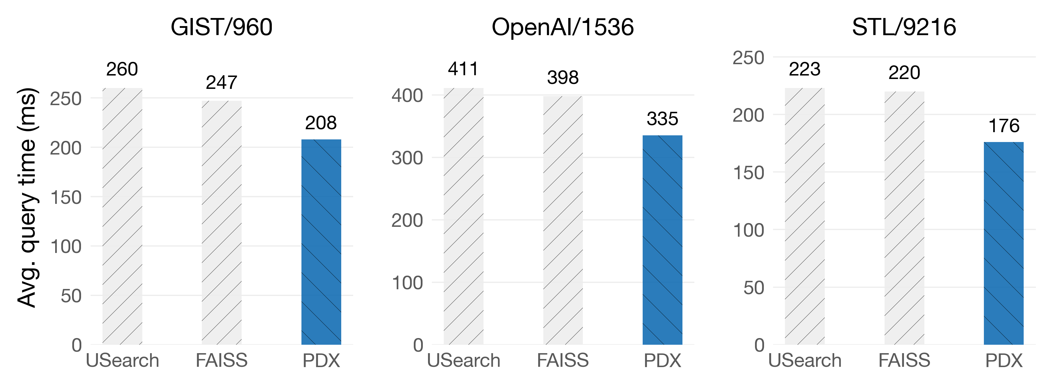
On Intel Sapphire Rapids
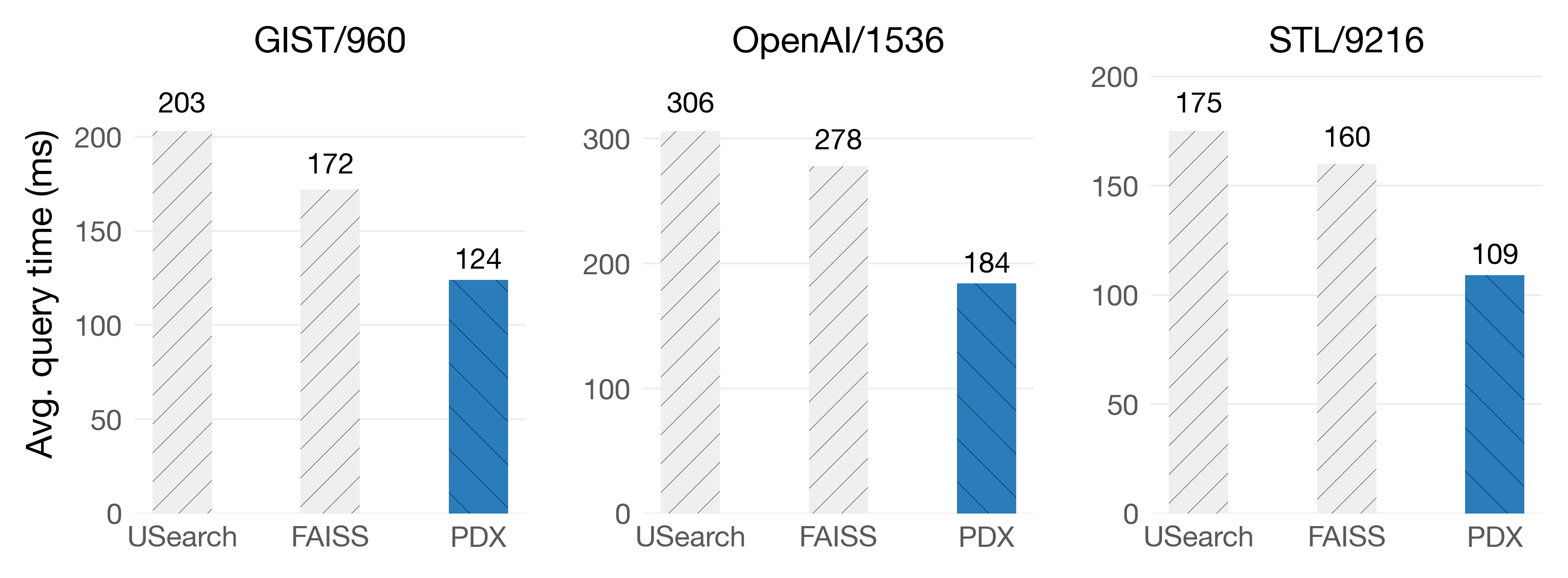
On Graviton4
On Graviton4, we get 34% faster queries on the OpenAI/1536 dataset!
But… is this all that the vertical layout has to offer? Of course not! PDX turns out to be the most suitable environment for pruning algorithms.
The power of pruning
LLMs produce vector embeddings of high dimensionalities (512, 768, 1024, 1536, and sometimes even more). This is challenging from the perspective of vector similarity search (VSS), as every extra vector adds more computational overhead and memory consumption. However, a few recent studies have proposed to prune dimensions during a search without sacrificing the search quality.
Pruning means avoiding checking all the dimensions of a vector to determine if it will make it onto the KNN of a query. Pruning speedup VSS as less data must be fetched and fewer computations must be done.
Pruning algorithms based on partial distance calculations work as follows: (i) Take the first △d dimensions from a vector (e.g., △d = 32). (ii) Calculate the partial distance between the vector and the query on the current △d dimensions. (iii) If the partial distance is higher than a pruning threshold (e.g., the distance of the current k-th neighbor of the query), there is no need to visit the remaining dimensions of the vector, as the L2 distance is monotonically increasing. Otherwise, take the following △d dimensions of the vector and go to step (ii).
On paper, this sounds great! We can potentially avoid millions of computations just by doing an extra evaluation every 32 dimensions. Unfortunately, this pruning strategy actually has a hard time being on par with SIMD-optimized kernels, like the ones in FAISS and SimSIMD. This is because distance calculations with SIMD are super powerful but also very brittle. Introducing an if-else statement to evaluate the current partial distance within the core work loop is detrimental to performance. So much that the performance of NOT pruning can be better than pruning in certain CPU microarchitectures.
Thankfully, PDX comes to the rescue of pruning algorithms!
The power of pruning + PDX
Aside from giving a nice speedup to distance kernels, PDX is also the perfect environment for pruning algorithms! Naturally, we needed to change how pruning works as a whole. Thus, we came up with PDXearch, our search framework for pruned vector search on PDX.
To explain PDXearch, let’s assume we have vectors indexed with an IVF index. Within every cluster, vectors are stored with the vertical layout. When a query arrives, some clusters are chosen for probing. Then, PDXearch goes as follows:
On the first cluster, we do a vertical linear-scan of the vectors. That is, we do not prune. With these distances, we build our top-K max-heap. The head of this heap is our pruning threshold. We call this the “START” phase.
On the following clusters:
- Visit the first △d dimensions of all the vectors in the cluster. Now, △d is not limited to 32. We can start as low as
△d = 2without compromising performance. - Calculate the partial distances between the query and the vectors on the current △d dimensions.
- Compare every partial distance to the pruning threshold and keep track of the number of vectors that have been pruned (n_pruned).
- Note that this comparison is done in a loop separated from the distance calculations, and it can be really fast by using a predicated comparison.
ifthe number of pruned vectors (n_pruned) is lower than 75% of the total vectors in the cluster, we go back to Step 2 with a higher △d.else, go back to Step 2, but now, only visit the dimensions of the not-yet pruned vectors.
Once we reach the last dimension, we merge the distances of the vectors that were not pruned to the top-K max-heap (if necessary).
Here is an illustration of the process:
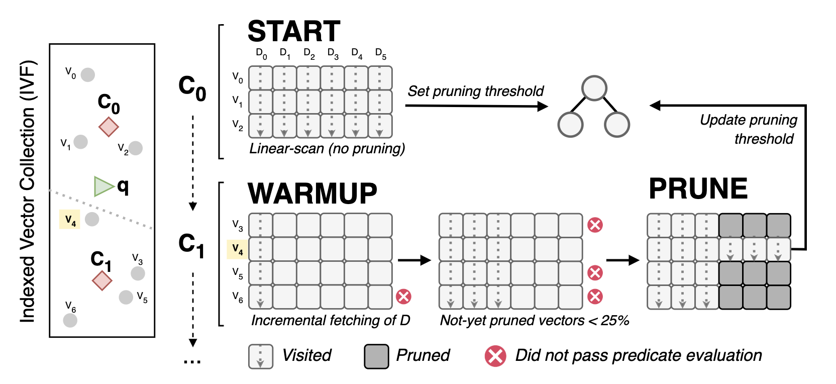
The PDXearch framework within an IVF index: A search happens dimension-by-dimension per IVF cluster. A linear scan is done in the first cluster (C0 in the figure) to set a pruning threshold. In the following blocks (C1), the search has two phases: WARMUP (keep scanning all vectors at incremental steps of D) and PRUNE (scan only the not-yet pruned vectors once they are few)
Perhaps the biggest question regarding this algorithm is: Why do you wait until a certain number of vectors are pruned to actually prune? This is because starting to prune vectors on PDX means to start jumping through memory to get the values of the remaining dimensions. Thus, if we begin to prune too early, PDX would be slower due to the jumping around memory, where also SIMD cannot be leveraged for the distance calculations.
Lucky for us, the behavior of the pruning rate is very predictable: Once pruning starts, it prunes exponentially fast! In other words, as soon as the algorithm starts discarding vectors, the majority of vectors in a block are going to be pruned in the following dimensions. You can see it is a sweet spot, which is query- and dataset-dependent.
Great! We have migrated pruning methods to the vertical layout. Is this now more efficient than SIMD-optimized distance kernels? Spoiler: It is.
Comparison with FAISS
We paired PDX with the current state-of-the-art pruning algorithms based on partial distance calculations (ADSampling and DDC). These algorithms rely on rotating the vector collection to achieve effective pruning. As I want to keep this post simple in terms of technical details, I recommend you take a look at the excellent paper of ADSampling to get the gist of how and why doing a random rotation to the collection works so well for pruning without sacrificing search quality.
As part of our publication, we also introduce our own pruning algorithm, PDX-BOND, which does not need a random rotation to perform well. This algorithm was also inspired by an idea presented in the mythical paper that inspired PDX.
Let’s go through the use cases in which PDXearch shines. For these, we show some single-threaded benchmarks running the examples available in our repository, which compare PDXearch performance to FAISS. We used r7iz.2xlarge (Intel SPR) and r8g.2xlarge (Graviton 4) AWS instances.
IVF Indexes
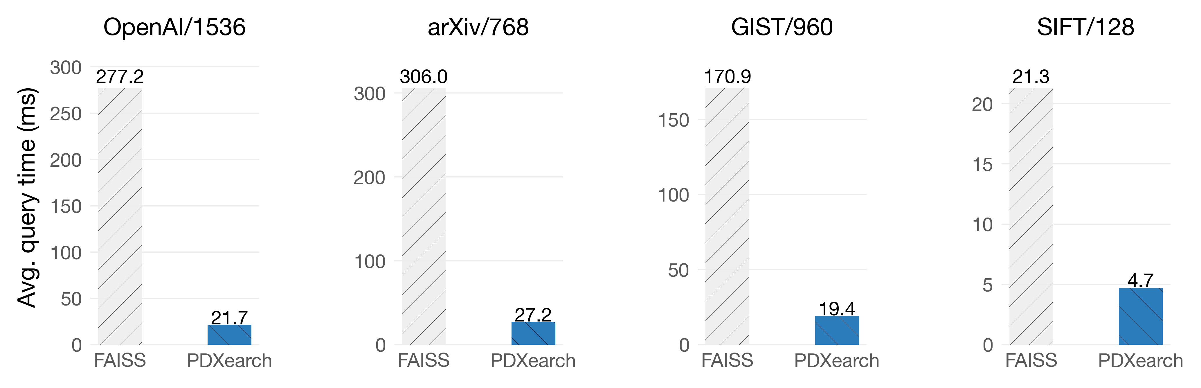
PDX paired with ADSampling on IVF indexes works great in most scenarios. On these benchmarks, both FAISS and PDXearch scan exactly the same vectors. We show results of the average query time (lower is better) on three datasets at three recall levels: R@10: 0.99 · 0.95 · 0.90.
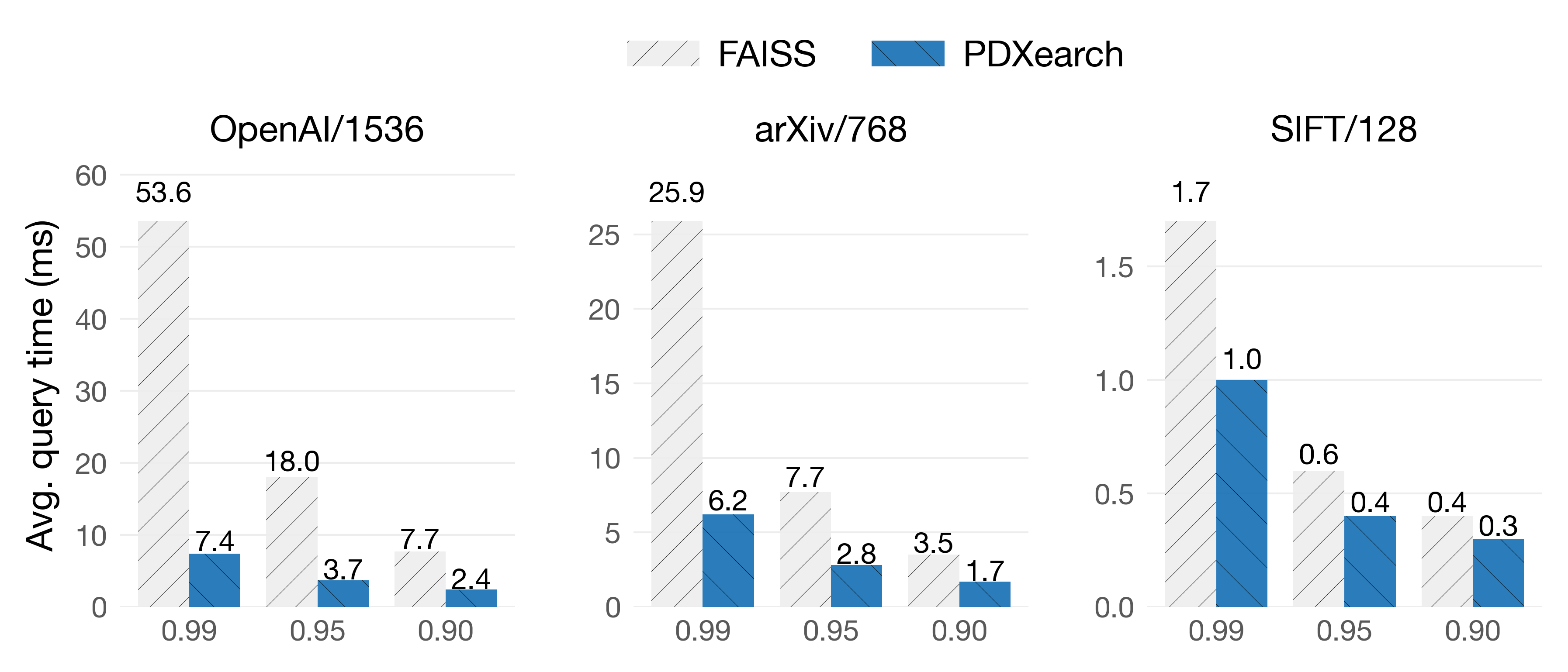
On Intel Sapphire Rapids
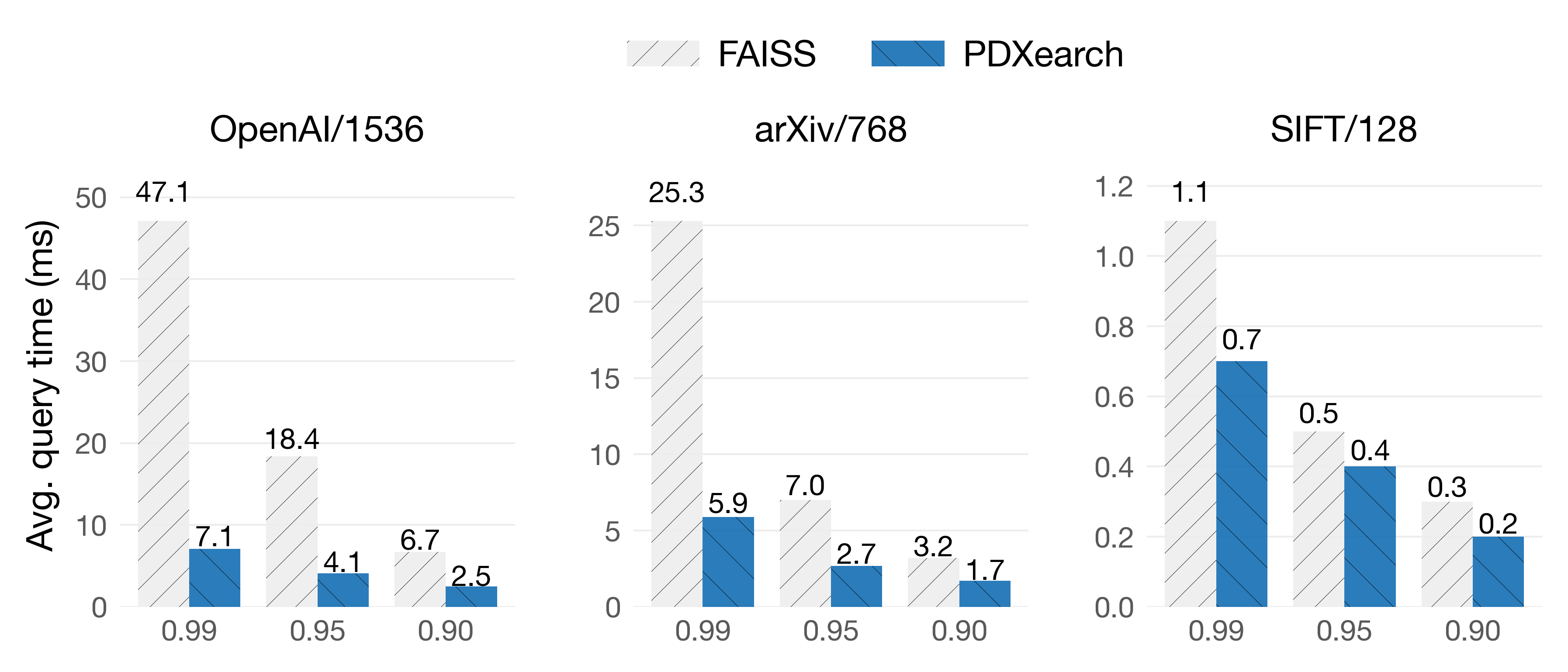
On Graviton4
In the OpenAI/1536 dataset, queries are 7.2x faster at 0.99 of recall! While on the SIFT/128 dataset, despite its lower dimensionality, queries still see speedups. As you can see, pruning algorithms are especially effective when vectors are of higher dimensionalities (d > 512) and high recalls are needed.
Exhaustive search + IVF
Exhaustive search means scanning all the vectors of the collection so that the answers to the query are the actual neighbors of the query. In PDX, building an IVF index can significantly improve the speed of exhaustive search (up to 13x!), even if the clustering is not super optimized.
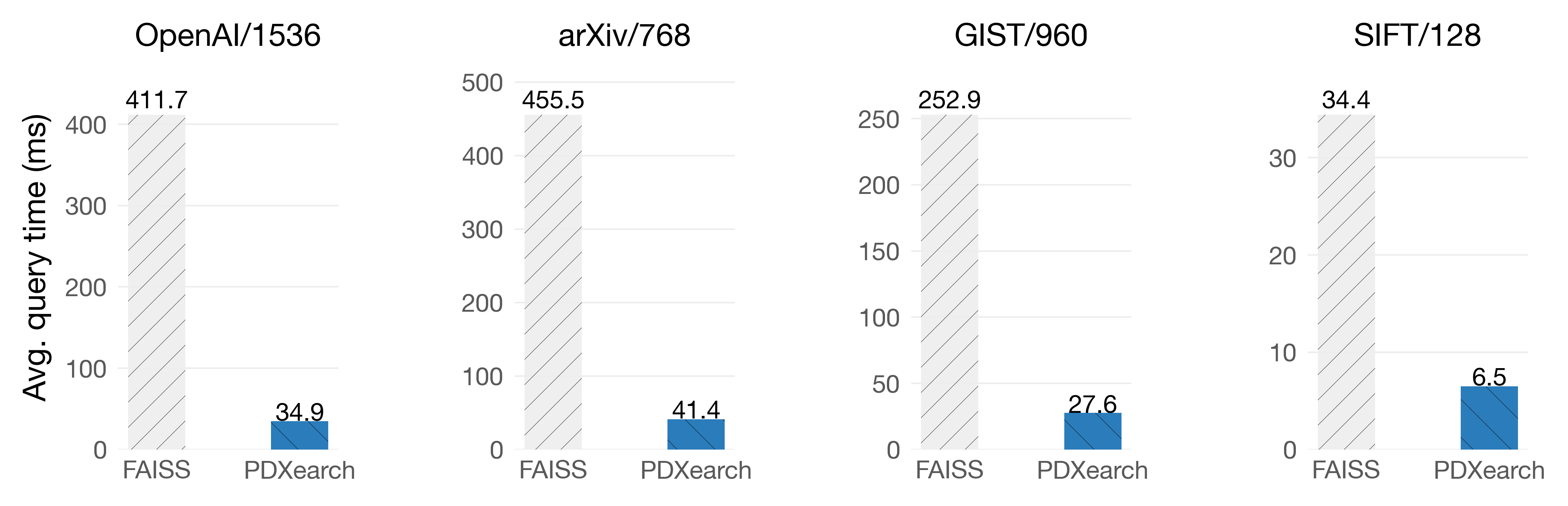
On Intel Sapphire Rapids
On Graviton4
The key observation here is that the exhaustive search can start with the most promising clusters thanks to the underlying IVF index. This will give us a pretty tight threshold to prune in the following ones. For example, let’s say we have 1024 clusters. Most of the KNNs of the query were probably on the first 128 clusters. In the other 896 clusters, the vectors are probably far away from the query. Therefore, the pruning algorithm does a good job of discarding all the vectors quickly. We may still find a better KNN in those 896 clusters, but most of the vectors are going to be pruned.
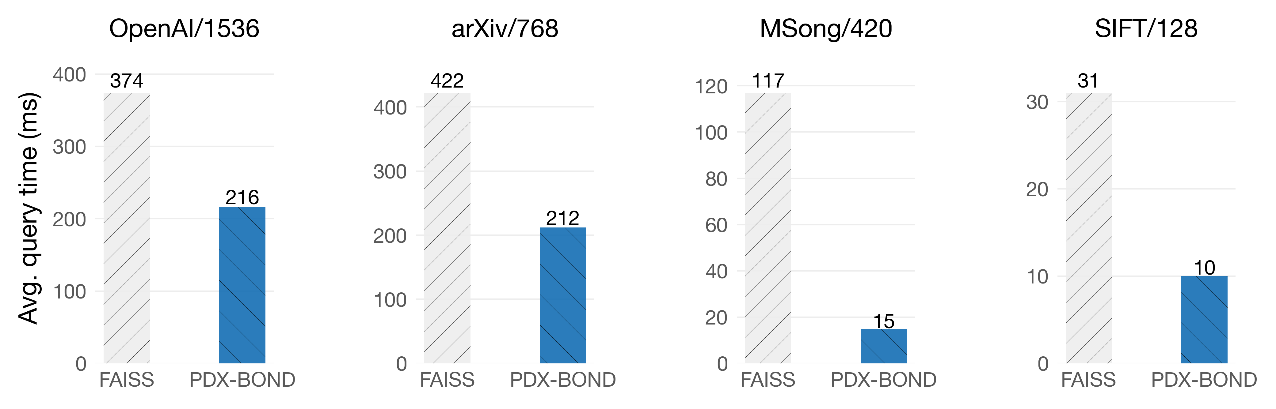
Exhaustive search without an index
With our pruning algorithm, PDX-BOND, you can do an exhaustive search without needing to rotate the vectors. Gains vary depending on the dimensions distribution.
On Intel Sapphire Rapids
Challenges of PDX
PDX is a young project. There are still a lot of questions in my mind that are pending to solve:
- Predicated queries: Modern Vector Databases support queries that do both VSS and relational queries at the same time. Depending on the selectivity of the relational filter, PDX could struggle. If the predicate has a low selection percentage, the bottleneck may not be in VSS. If it has a high selection percentage, we can do PDXearch on all the vectors. But, if the predicate has an in-between selectivity, PDX could be in trouble. A possible solution would be IVF indexes that are also partitioned by these relational attributes.
- 1-to-1 similarity search (a subset of the problem above): PDX will be slower than horizontal kernels if there are less than 16 vectors to be evaluated (technically, it would depend on the SIMD register width of the CPU). However, if that is the case, the bottleneck of the application may not be in the VSS.
- Quantized vectors: Going from
float32tofloat16oruint8in PDX will not be trivial. The problem is that the distance accumulation must happen in thefloat32oruint32domain. However, there is noFMADDinstruction (or, in reality, any SIMD instruction) that operates on individualuint8values and accumulates onuint32. Fortunately, we have found a workaround for this with promising results, still outperforming the symmetric distance kernels in SimSIMD! So, keep tuned :) - Overhead of the pruning phase: When PDX starts the actual pruning, the algorithm begins jumping through memory. A SIMD
GATHERhelps to speed up this phase by 20% on Intel SPR. However, we are exploring ideas on using a hybrid layout that stores some dimensions with PDX, and the rest with the horizontal layout can help even further. Dual storage (both vertical and horizontal) would also be a solution to speed up the pruning phase and support predicated queries of low selectivity. - Other distance metrics: Pruning works because L2 is a monotonically increasing metric. However, not all distance metrics are. Luckily, for the most common distance metrics, there are mathematical shenanigans we can use to keep using L2 and keep pruning those vectors.
- HNSW indexes: For PDX to work in HNSW, we need a data layout similar to the ones proposed in Starling or AiSAQ, in which neighborhoods of the graph are stored and fetched in blocks. This is not a priority, as we believe that IVF indexes are cooler :)
At CWI, we are currently looking for MSc. students to help us develop PDX! If you are interested in PDX and are looking for thesis projects, reach out at [email protected]
Closing remarks
We believe that the core idea of pruning algorithms like ADSampling, DDC, and DADE is the next leap in VSS, as the distance calculation cannot be avoided in any VSS setting. With PDX, pruning algorithms are the clear winners over SIMD-optimized kernels in any microarchitecture and at any dimensionality of vectors.
Pruning algorithms perform exceptionally well when the dimensionality of the vectors is high and when high recalls are needed. In fact, on the sizes of datasets we used (1M - 2.2M), the performance of an IVF index search that prunes is actually pretty close to that of HNSW (more on this in a future post!). This makes PDX+Pruning a very attractive alternative to being fast without having to build a graph index.
For now, the speedups of PDX (both with and without pruning) are not free: one has to change the data layout of the vectors. As we have mentioned, this can be a problem, depending on the type of vector workload. However, we are optimistic that we can overcome these challenges and provide a super-fast vector search system based on PDX.
This blog post was a very condensed summary of our scientific publication. If you are interested in all the intricacies and details, you should give it a read! Here, we show benchmarks of PDXearch in 4 microarchitectures: Intel SPR, Zen4, Zen3, and Graviton4. Also, you will find a comparison against pruning algorithms in the horizontal layout. You can also check our GitHub repository to replicate our benchmarks and try PDX with your own data: https://github.com/cwida/PDX.